Decision Making Needs Modeling Intervention Effects
Review of treatment effect estimation techniques
Problem with ML
Predictive machine learning models are built to improve decision making process. Usually they are embedded in complex decision logic. There are many processes that are intervened by us based on the predictions our ML model makes. For instance, consider churn prevention problem.
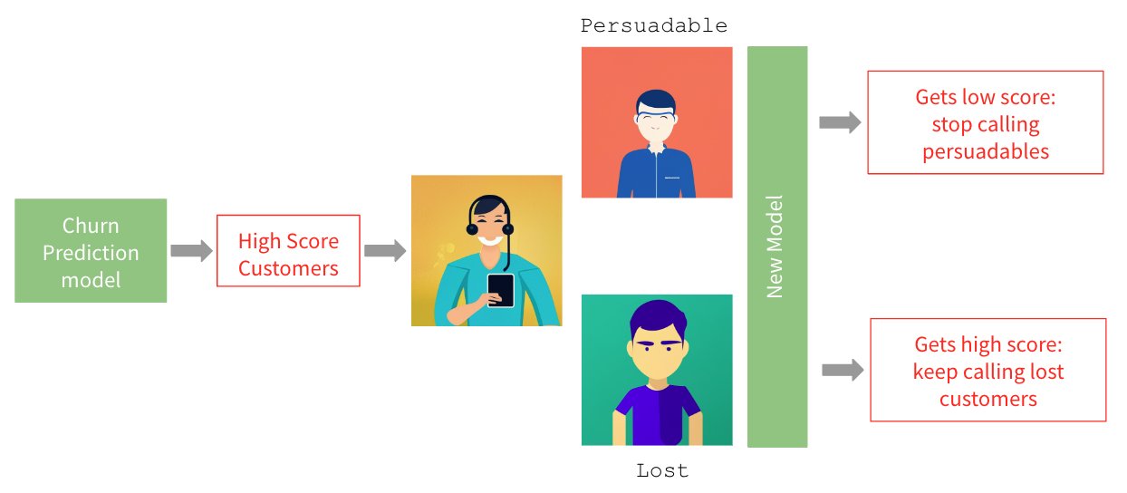
We build a churn prediction model, then we score the entire customer base, customers with the highest churn scores are identified and customer experience team sends them relevant offers retain them. After receiving offers some of them do not churn but some leave anyway. Few months later the churn model needs to be retrained on the new sample where persuadable customers (the ones that were contacted and stayed) are labeled as 0, while the lost ones (the ones that were contacted but left) are labeled as 1. Therefore former gets low score whereas the latter gets high score. So the new model learns to stop calling persuadable customers and keep calling lost customers. None of them is a decision we want to make. What this use case teaches us is that
One should estimate the intervention effect or, in this case, probability of churn given intervention instead of simply retraining the model.
In the following we review algorithms for modeling intervention (treatment) effects. But before that let’s talk about another problem of ML which is “causation is not the same as correlation”. Let’s demonstrate this in case of two very basic causal DAGs, Fork and Collider.

Fork describes a process when a a single variable Z is affecting both X and Y and therefore they appear correlated even though there is is no causal link between them.
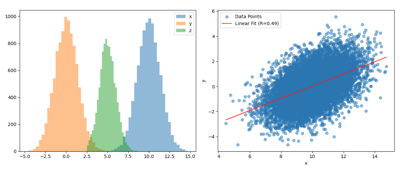
The spurious correlation is gone only after conditioning both of them on Z.
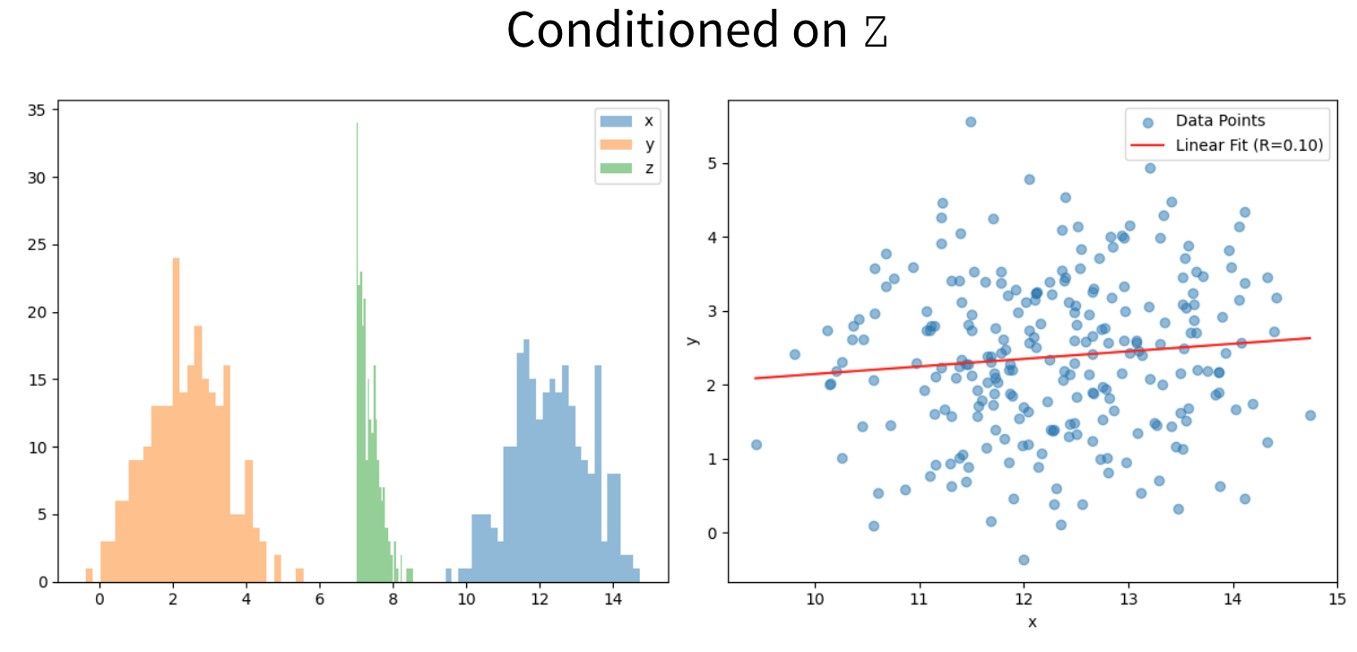
In Collider X and Y are not causally linked but they both affect Z. One doesn’t observe any correlation between X and Y, as it should be.
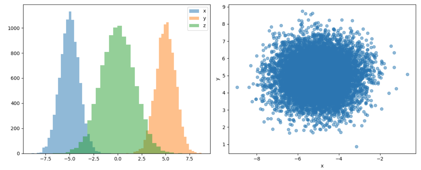
But conditioning them on Z leads to a large $R^2$.
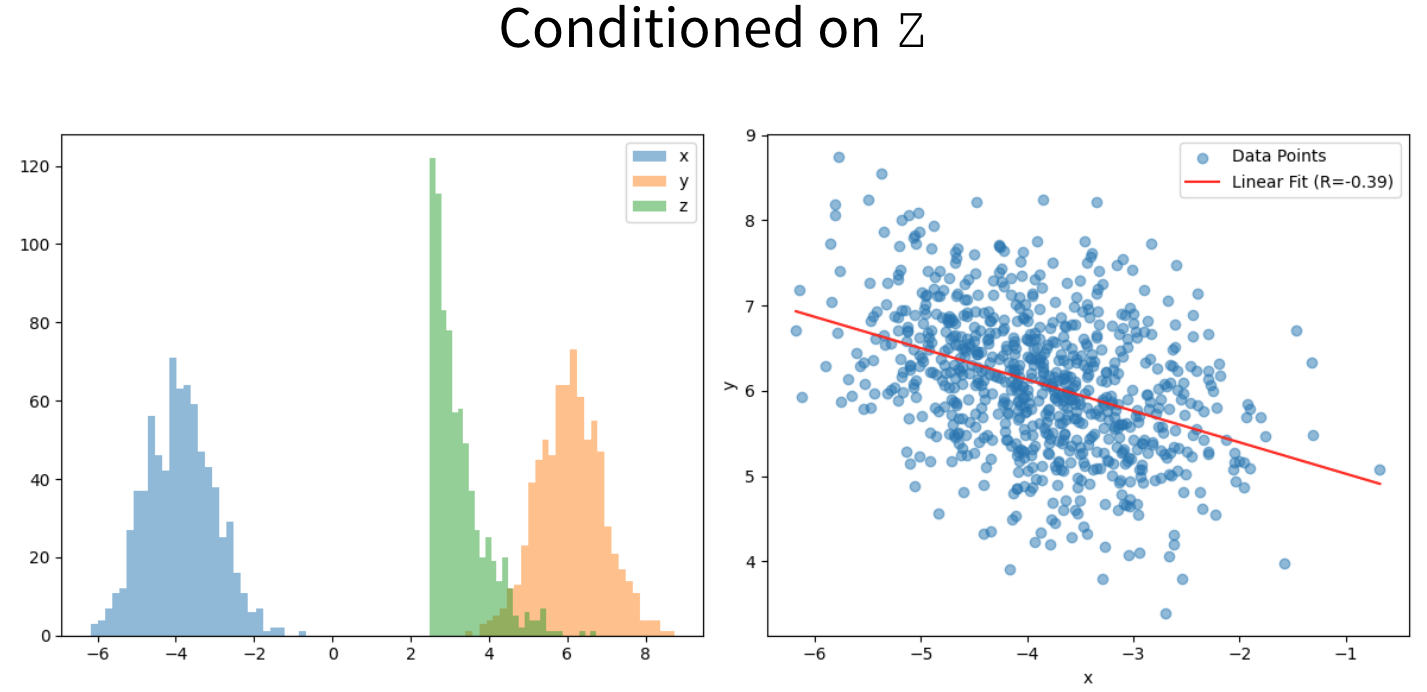
Therefore, ignoring causal links can also lead us to wrong decisions as they would be based on the spurious correlations.
Definitions
Estimating a treatment effect implies answering what if… question or, in technical terms, estimating the corresponding counterfactual. Counterfactual refers to the value of the parameter of interest if intervention had not occur. So in the case of the churn use case, that would be the scenario when we never communicate with the customers. Another important concept is the treatment effect, which is the difference between the value of the parameter for the treated unit and the value the parameter for the treated unit would have had if we had not applied any treatment, Eq. 1.
\begin{equation} TE = Y_T(t=1;W=1)-Y_T(t=1;W=0) \end{equation}
Y is the variable of interest where T stands for treatment group, t is a binary variable indicating whether it is measured in pre ($t=0$)- or post-intervention ($t=1$) period and W is also binary telling us whether treatment is applied or not. So by definition the second term in Eq.1 is counterfactual. Usually we want to calculate conditional average treatment effect given in Eq. 2.
\begin{equation} CATE = E[Y_T(t=1;W=1)-Y_T(t=1;W=0)|X] \end{equation}
Another term for the treatment effect coming from the marketing literature is uplift. It is used in the context of the interventions applied to a customer base.
Algorithms for Treatment Effect Estimation
Difference in Differences (DiD)
So basically problem of treatment effect reduces to the counterfactual estimation because the first term in Eq. 2 is observed. There are two naive approximations for the counterfactual. The first one is to replace it with the value of $Y_T$ before the intervention.
\[CATE = E[Y_T(t=1;W=1)-Y_T(t=0;W=0)|X]\]But this is not a good approximation because it assumes that there is no trend or seasonality in the time series and it changes only due the intervention. The second approximation is to utilize the control group in the post intervention period.
\[CATE = E[Y_T(t=1;W=1)-Y_C(t=1;W=0)|X]\]But this approximation assumes that the control group is very similar to the treatment group in the pre-intervention period and would have remained similar if no treatment had been applied. That is also a strong assumption. Usually what’s used in practice is the combination of these two approximations resulting in the DiD estimator. So, counterfactual term is approximated with
\[\begin{align*} E[Y_T(t=1;W=0)|X]=&E[Y_T(t=0;W=0)|X]+\\ &+(E[Y_C(t=1;W=0)|X]-E[Y_C(t=0;W=0)|X]). \end{align*}\]Plugging it into the equation of CATE yields
\[\begin{align*} CATE = &(E[Y_T(t=1;W=1)|X] - E[Y_T(t=0;W=0)|X])-\\ &-(E[Y_C(t=1;W=0)|X]-E[Y_C(t=0;W=0)|X]). \end{align*}\]The first term is the difference between $Y_T$ values before and after intervention which is the treatment effect plus the change that would have occurred anyway. To cancel out the latter component the second term is subtracted which is a difference between $Y_C$ values before and after intervention. In other words we assume that the natural change that would have occurred in the treatment group is the same as in the control group. What if treatment and control time series have different scales? If this is the case let’s approximate the counterfactual using
\[\begin{align*} E[Y_T(t=1;W=0)|X]=E[Y_T(t=0;W=0)|X]\cdot \frac{E[Y_C(t=1;W=0)|X]}{E[Y_C(t=0;W=0)|X]} \end{align*}\]resulting in
\[\begin{align*} CATE &= (E[Y_T(t=1;W=1)|X] - E[Y_T(t=0;W=0)|X])-\\ &-\frac{E[Y_T(t=0;W=0|X)]}{E[Y_C(t=0;W=0|X)]}\cdot(E[Y_C(t=1;W=0)|X]-E[Y_C(t=0;W=0)|X]) \end{align*}\]more general expression in a sense that it reduces to the previous formula if the expectation of the treatment and control group values before the intervention are equal. Hence, to resolve issue of having different scales in the treatment and control time series ratio between pre- and post-intervention control group values is used instead of the absolute difference.
Synthetic Control Brodersen et al., Annals of Applied Statistics (2015)
DiD requires treatment and control time series to have parallel trends and, in general, to be similar. This is quite strong requirement which is dropped by the synthetic control approach. Instead of finding a control time series very similar to the treated one let’s train a model on the bunch of untreated time series with output variable being the treated time series before the intervention. If the trained model has a good performance and accurately predicts the treated time series it can serve us as the control group. The model predictions in the post-intervention period represents counterfactual estimations. This is a very trivial but powerful idea. We don’t have to find time series similar to the treatment group, the only requirement is that the intervention does not affect them and they need to be predictive of the treatment time series.

Fig. 1 depicts this idea. $Y$ is the treated time series while $X_1$ and $X_2$ are input to the model that tries to predict $Y$. The dashed vertical line denotes the intervention. The solid blue is the fitted line whereas dashed blue line represents forecasts after the intervention. Therefore CATE would be the difference between solid black and dashed blue lines.
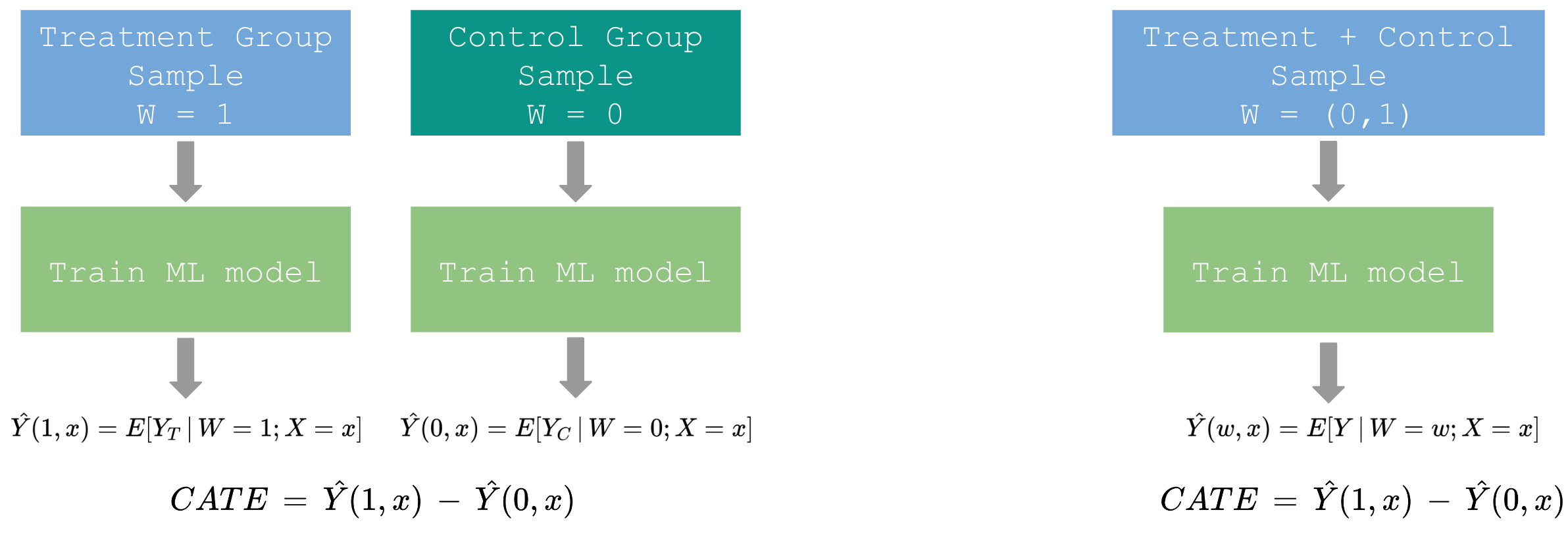
2-Model Approach S. Athey and G. W. Imbens, Machine learning methods for estimating heterogeneous causal effects, stat, 1050:5, 2015b.
Another way of estimating CATE is to train two models on the treatment and the control group samples, respectively. Their predictions are estimates of the two terms in the definition of CATE in Eq. 2. This method can be reduced to the 1-model approach by combining treatment and control samples and adding W=(0,1) to the combined sample as one of the features.
Target Transformation Approach
The disadvantage of the previous technique is that models have their own errors and after subtracting their predictions we are not guaranteed that those errors cancel each other. Most likely the treatment effect has even bigger error. To avoid it we introduce an approach which models CATE explicitly. Let’s first describe it in the case of the binary outcome followed by the general case.
Binary Target Jaskowski M., & Jaroszewicz S., "Uplift modeling for clinical trial data." ICML Workshop on Clinical Data Analysis. Vol. 46. 2012
CATE for the discrete target variable is defined in the following way
\[CATE = P(Y=1|X;W=1)-P(Y=1|X;W=0)\]So it’s simply a probability of success in the treatment group minus the probability of success in the control group. Now introduce a new variable Z
\[Z=Y\cdot W+(1-Y)\cdot (1-W).\]Here is the list of all possible values of Z:
\[Z = \begin{cases} 1 &\text{Y=1, $W=1 $}\\ 1 &\text{Y=0, $W=0 $}\\ 0 &\text{Y=0, $W=1 $}\\ 0 &\text{Y=1, $W=0 $}\\ \end{cases}\]Let’s compute the conditional probability of Z being 1.
\[P(Z=1|X)=P(Y=1|X;W=1)P(W=1|X)+P(Y=1|X;W=0)P(W=0|X)\]Now we make an assumption of balanced treatment (whether an object is treated or not does not depend on $X$ and the probability of being treated is the same as the one of not being treated)
\[P(W=1|X)=P(W=0|X)=1/2\]which simplifies the latter equation further and gives
\[P(Y=1|X;W=1)-P(Y=1|X;W=0)=2P(Z=1|X)-1\]where left hand side is the definition of CATE. Therefore, modeling variable Z is the same as modeling uplift explicitly.
General Case S. Athey and G. W. Imbens, Machine learning methods for estimating heterogeneous causal effects, stat, 1050:5, 2015b.
In the previous section we made assumption of balanced treatment, meaning equal treatment and control groups, which, in general, doesn’t hold in practice. Also $W$ being independent of $X$ can’t be achieved unless we have completely randomized process. To drop that assumption consider another transformation of the outcome variable which does not have to be binary anymore.
\[Z=Y(W=1)\cdot \frac{W}{p(X)}-Y(W=0)\cdot \frac{1-W}{1-p(X)}\]where
\[p(X)=P(W=1|X)\]is a propensity score (this idea is similar to the inverse propensity weighting approach). Let’s compute the expectation value of Z as we did in the previous section.
\[E[Z|X]=\frac{E[Y(W=1)\cdot W|X]}{p(X)}-\frac{E[Y(W=0)\cdot (1-W)]}{1-p(X)}\]Conditional Independence Assumption or Unconfoundedness (whether object is treated or not does not depend on the outcome)
\[W \perp (Y(W=1), Y(W=0))|X\]reduces the equation to the definition of CATE
\[E[Z|X]=E[Y(W=1)|X]-E[Y(W=0)|X].\]Here we used the following relationship
\[E[W|X]=p(X).\]Again, modeling Z gives the treatment effect directly.
Summary
As we discussed in the introduction it is important to incorporate treatments in the modeling process otherwise we would make wrong decisions. This was the motivation for reviewing four different approaches for modeling the treatment effect. I think it is natural to group them into two different groups.
| Uplift Estimation | Uplift Prediction |
|---|---|
| DiD Estimator | 2-Model Approach |
| Synthetic Control | Targete Transformation Method |
DiD and Synthetic Control are used when intervention already occurred, post-intervention values of the treatment group are already observed and we want to estimate the effect. But if we want to predict the uplift before the intervention 2-Model and Target Transformation approaches are relevant. And lastly, Synthetic Control is the only method out of these four which allows using time series of completely different variables than the one in the treatment group as a control and additionally, unlike DiD, it allows using a dissimilar time series of the same variable as a control.