Prediction Intervals for Aggregated Forecasts
A framework for constructing prediction intervals
Intro
I won’t go into details about why prediction intervals are important, we all know that. I just want to introduce a framework that will allow us to estimate a prediction interval for a single forecast, and then we will generalize it for aggregated forecasts. I started thinking about this problem when I was working on a sales forecasting model earlier this year. The model produced monthly forecasts, but the clients were interested in aggregated forecasts, such as annual sales of a store or forecasted annual sales for the entire shopping mall. I realized that I needed a way to estimate the prediction interval for aggregated forecasts, given that I only had a model that produced monthly forecasts.
Distribution-free Approach
There are many approaches to building prediction intervals. Most of them are based on the residuals assumed that they are normally distributed. There are some fancy formulas that allow you to construct prediction intervals based on this normality assumption. However, we know that this assumption is often unrealistic and doesn’t hold in practice. I wanted to have a method that is distribution-free, so I decided to use a technique based on the bootstrapping approach. The basic idea is to simulate future paths of the variable of interest. This will allow us to estimate the distribution of the variable at any future time point. The technique can be used for supervised learning algorithms as well as time series algorithms.
Simulating Future Paths
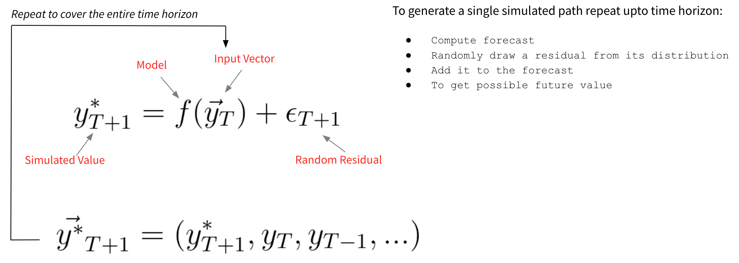
To generate a simulated path, we start with a forecast at the first time point in the horizon, \(T+1\), draw a random residual from the residual distribution and add it to the forecast. This gives us the first simulated value, \(y^*_{T+1}\). We then use the first simulated value as the input to the model to generate a forecast for the next time point in the horizon. We repeat this process until we have generated a sequence of simulated values for all of the future time points. This process is repeated multiple times to generate multiple simulated paths. This will give us a distribution of the variable of interesty at any future time point which is used to construct prediction intervals.

Aggregation Across Different Dimensions
We consider two types of aggregations:
- Aggregation across time axis is the process of combining forecasts for different time points into a single forecast. For example, if you have monthly forecasts for a year, you can aggregate them to get an annual forecast.
- Aggregation across time series is the process of combining forecasts for different time series into a single forecast. For example, if you have forecasts for sales of different products, you can aggregate them to get a forecast for total sales. Our method can be used to estimate prediction intervals for both, aggregation across time and aggregation across time series.
Aggregation Across Time
For each simulated path, aggregate the monthly forecasts to obtain an annual forecast. This can be done by simply summing the monthly forecasts for each year (see equation below). As a result we are left with an array of \(N\) (number of simulated paths) elements for a given year, \((y_{1,year}, y_{2,year},..., y_{N,year})\). Estimate the lower and upper bounds of the prediction interval at the desired confidence level by computing \((1-\alpha)/2\)-th and \((1+\alpha)/2\)-th quantiles of the resulting distribution.
\[y^*_{s, 2027} = \sum^{12}_{m=1} y^*_{s,m/2027}\]Aggregation Across Time Series
To estimate a prediction interval for an aggregated forecast across time series do a cross-section of the simulated paths for each time series at the time point of interest. Which gives us \(T\) (number of time series) arrays of length \(N\) (number of simulated paths in a single time series). Each array is a distribution of \(y\) at that time point. Therefore, we can say that we have a set of distributions of \(T\) random variables and the goal is to estimate the distribution of the sum of those random variables given that the distribution for each of them is known. One approach to do that is convolution but becomes infeasible when the number of random variables (time series) is large. More scalable and fast approach is Monte Carlo simulation: these arrays/distributions are put together in a matrix with columns being a distribution corresponding to a single time series. So, the matrix has an \(N \times T\) shape (\(N\) rows because there are \(N\) elements in a distribution since there are \(N\) paths, \(T\) columns - because we have \(T\) time series to aggregate). Then we sum the matrix entries horizontally resulting in the array of length \(N\) which is the estimation of the distribution of the aggregated forecasts. Estimate the lower and upper bounds of the prediction interval at the desired confidence level by computing quantiles of the resulting distribution.
\[\begin{bmatrix} y^{*,1}_{1} & y^{*,2}_{1} & y^{*,3}_{1} & \cdots & y^{*,T}_{1} \\ y^{*,1}_{2} & y^{*,2}_{2} & y^{*,3}_{2} & \cdots & y^{*,T}_{2} \\ \vdots & \vdots & \vdots & \ddots & \vdots \\ y^{*,1}_{N} & y^{*,2}_{N} & y^{*,3}_{N} & \cdots & y^{*,T}_{N} \\ \end{bmatrix} \begin{matrix} \\ \stackrel{\sum_t}{\Longrightarrow} \\ \\ \end{matrix} \begin{bmatrix} Y^*_{1} \\ Y^*_{2} \\ \vdots \\ Y^*_{N} \end{bmatrix}\]Fit Prophet into the Framework
Prophet has three main components: trend, seasonality and holidays. Trend is a major driver of the model. Prophet is a special algorithm in the sense that once a model is fitted, the trend has a constant slope and thus the Prophet model is blind, insensitive to the modifications we do to the input vector (adding a residual to the forecast). In order to generate the path one has to refit Prophet every time we update the input vector in order for the trend slope to be updated accordingly. But this approach is time consuming because the model needs to be fitted as many times as the number of time points in the forecasting horizon.
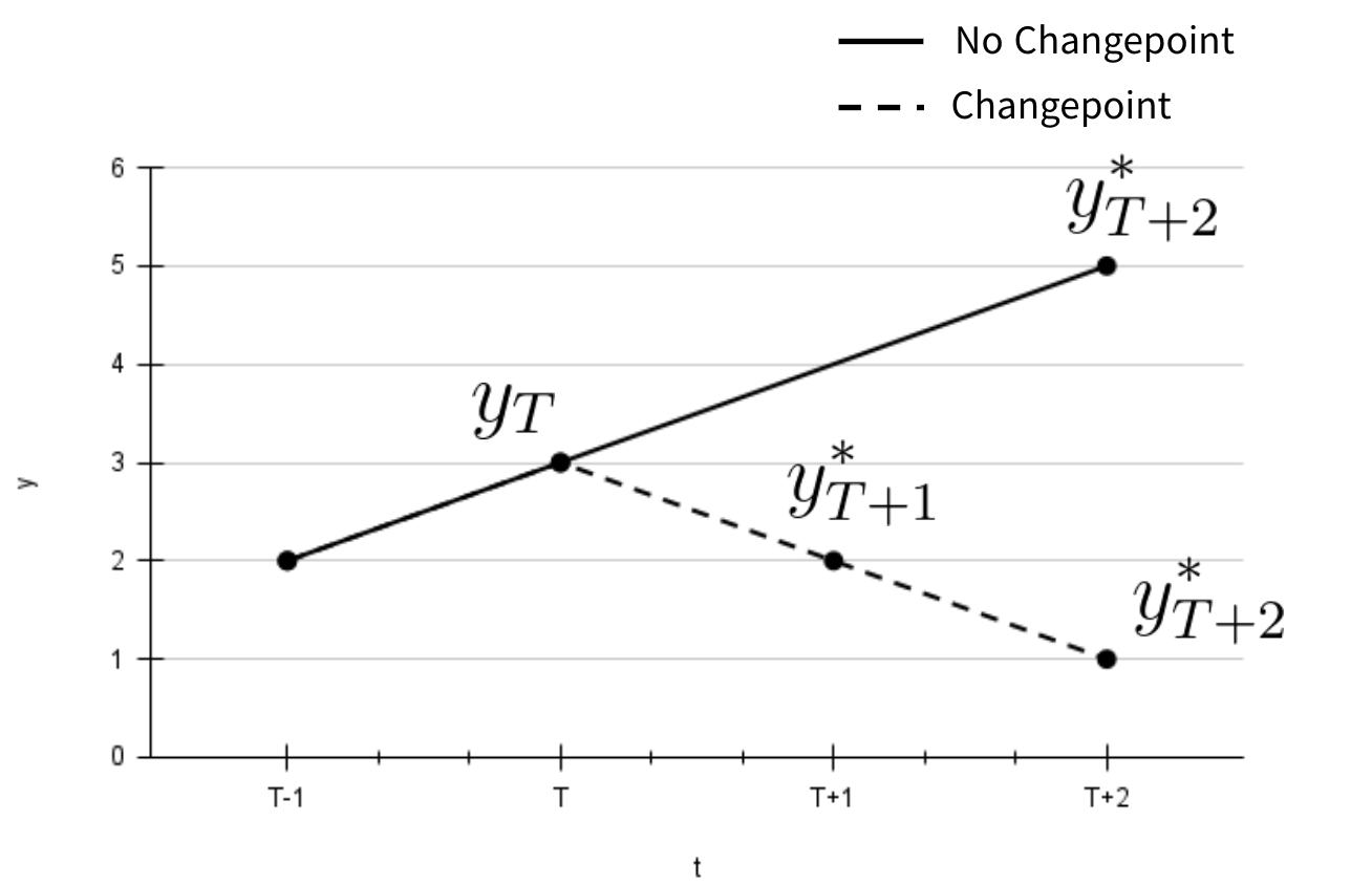
To avoid that we make an approximation. We assume that the perturbation of the forecast affects only the trend component, others remain the same. We also need to remember how a trend is learned. First Prophet identifies change points in the original time series and the trend is simply a piecewise linear curve connecting all pairs of neighboring change points. So the slope of the trend is allowed to change only after it passes the change point otherwise it is constant.
We utilize these ideas to generate a future path in the case of the Prophet model. First we need to come up with a way to check whether a simulated point is a change point or not. To do that we look at the change points Prophet identified from the original time series and calculate the smallest change in the trend components observed at those historical change points. After we simulate a future value, say, \(y^*_{T+1}\) , we check whether the previous point (in this case it would be \(y_T\), this is not a simulated point as it is the last value in the time series) is a change point. It is a change point if a change in trend component at that point is greater or equal to the observed smallest change at the historical change points. In such case trend is updated and becomes a line connecting \(y_T\) and \(y^*_{T+1}\) Otherwise the slope of the trend remains the same. This is how the trend is simulated for future values. In order to reconstruct original values \(y_t\) we add seasonality and holiday components to the simulated trend values (remember we assume that only trend is affected in the path simulation process and seasonality and holiday components are already estimated by Prophet for the entire horizon).

Simulations
Here we show some examples for prediction intervals constructed for the Prophet model. The first graph simply shows simulated paths for a time series. The second is with prediction intervals without any aggregation for the same time series. The next graph shows prediction intervals for annual aggregation. The fourth one shows prediction intervals for the forecasts that are the sum of the forecasts computed by different multiple models. And finally prediction intervals in the case of both types of aggregations: sum of the annual forecasts coming from different models.


Summary
The benefit of simulated path based approach for calculating prediction intervals is that it is distribution-free, generalizable for aggregated forecasts, easy to implement and it is fast. What it lacks is drift adaptation mechanism. We also made an approximation but that is Prophet specific. No need to make similar approximation if another algorithm is used for time series modeling.