Cross-Validation Estimator
Discussing the variance of the cross-validation estimator
Notations:
- \(m\) - metric
- \(K\) - number of folds
- \(N\) - number of different training sample realizations (drawn from the true population)
- \(\overline{m^n}\) - average metric (over \(K\) folds) for a given training sample realization
- \(Var(m^n_k)\) - variance of a metric over \(K\) folds for a given training sample realization
- \(Var(\overline{m^n})\) - variance of an average metric (over different training sample realizations)
- \(Var(m)\) - True/population variance of a metric
Bias
The goal of the cross-validation is to estimate the mean of a metric, \(\overline{m}\) and its variance, \(Var(m)\). Cross-validation gives a pessimistically biased estimate of a performance because most statistical models will improve if the training set is made larger. However, Leave-one-out cross-validation (LOOCV) is approximately unbiased, because the difference in size between the training set used in each fold and the entire dataset is only a single instance.
Variance
Intra-fold variance of a metric \(Var(m^n_k)\) is affected by the sample size as well as how diverse the sample is or in other words how different are validation folds from each other. The folds can be quite different easily in the low data regime if there are some instabilities in the sample, like outliers (for instance, if a given validation fold is very different from the training fold the value of \(m^n_k\) can be very different from the other values and thus will increase its variance). To factor out the sample diversity/instabilities from the estimation of \(Var(m)\) cross-validation is repeated \(N\) times (\(N\) is a large number, say, 5000) with different training samples. As a result we get the \(N\) number of \(\overline{m^n}\) allowing us to compute the mean of means and the variance of means, \(Var(\overline{m^n})\) and that is what is usually referred to when discussing the variation of the CV estimator. If training samples are independent \(Var(\overline{m^n})\) is lower than that in the case of the correlated training samples based on the argument mentioned below.
Effect of Model Stability
Before we dive into the details one should mention that CV does a good job if we are dealing with large samples but small sample regime (e.g. 40-60 records) is a different story. Number of folds and instabilities have a prominent impact on the metric estimations in the latter scenario.
Intuitively one thinks that with increasing \(K\) we get more overlapped training samples and thus almost the same models within CV, training folds become highly correlated. They make similar predictions (almost the same prediction if \(K\) is very large, for example, if \(K\) is the same as the number of data points which corresponds to LOOCV) for a given validation sample. Therefore these estimates of a metric are not independent, they are correlated and consequently lead to higher variance, \(Var(\overline{m^n})\) [ref] (why the mean of a correlated data has larger variance than that of the independent one is explained here).
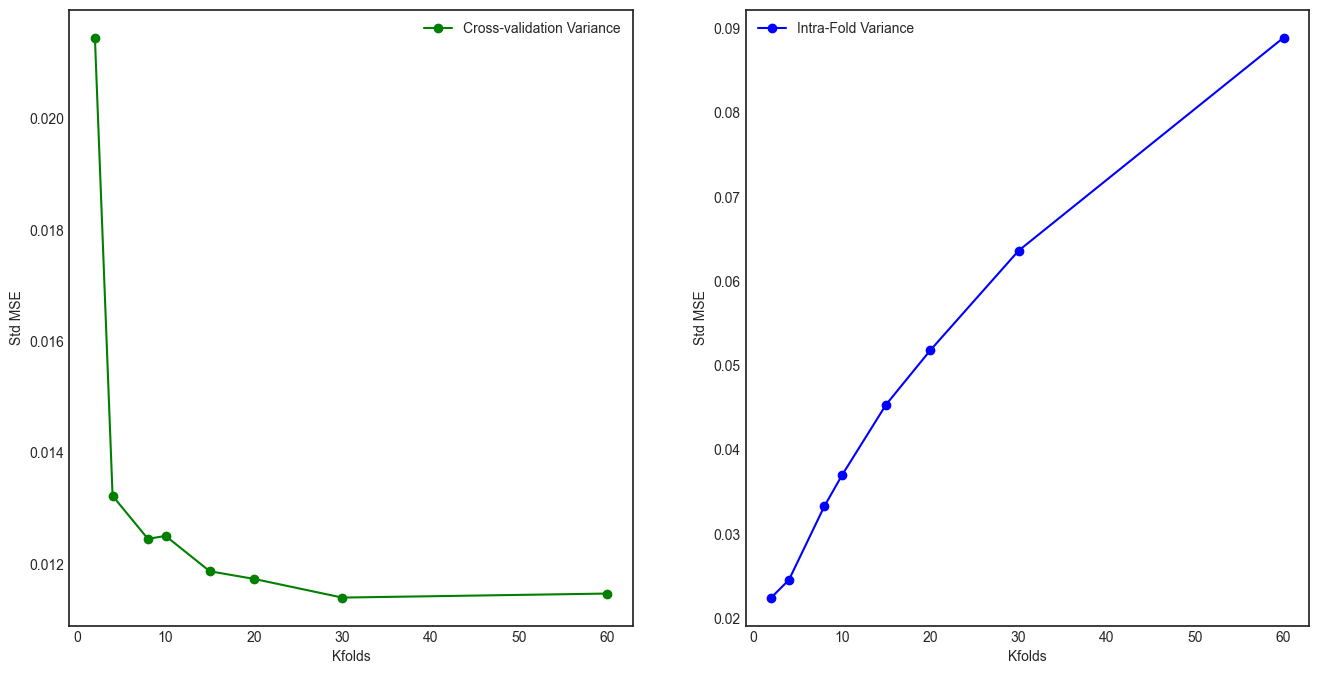
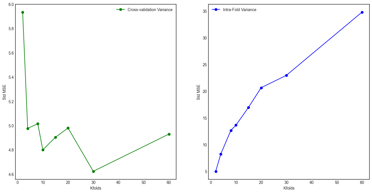
On the other hand one can show empirically that \(Var(\overline{m^n})\) doesn’t always increase with increasing \(K\) rather it depends on the stability of a model and a sample. If we are given a sample with no instabilities and a model is also stable1 \(Var(\overline{m^n})\) goes down with increasing \(K\) (LOOCV gives minimum or almost minimum variance) (see Fig. 1) while for the unstable case it reaches minimum for some intermediate value of \(K\) (LOOCV is not minimum anymore) [ref]. So the difference is in the high \(K\) region (see Fig. 2)2.


In general the variance is smaller in a stable environment compared to the unstable one. In the stable environment a given training sample is representative of the true distribution and thus \(\overline{m^n}\) is going to have similar values for different realizations of the training sample resulting in lower variance compared to the unstable scenario. In the latter case a given realization of the training sample is not representative of the underlying distribution. Imagine there are some instabilities in the sample, say, outliers. In the small data regime they may have a big influence on the model. For instance, if there are no outliers in the current realization of a sample (say, when \(n=1\)) we get stable model that behaves differently compared to the model we get, let’s say, in the next iteration (\(n=2\)) because in that realization outliers are present which is causing the fitted function to become more wavy/fluctuating. Due to that reason, outputs of these two models (\(n=1\) vs \(n=2\)) are going to be different and therefore there is larger difference between \(\overline{m^1}\) and \(\overline{m^2}\) leading to the higher variance, \(Var(\overline{m^n})\).
In the low data regime \(Var(\overline{m^n})\) is large for smaller \(K\) values in both cases, stable and unstable environments. That is because when \(K\) is small the training fold becomes smaller and the model becomes very unstable as it is more sensitive to any noise/sampling artifacts in the particular training sample used [ref].
| Model | With Increasing K |
|---|---|
| Stable | \(Var(m^n_k)\) increases, \(Var(\overline{m^n})\) decreases |
| Unstable | \(Var(m^n_k)\) increases, \(Var(\overline{m^n})\) has U shape (first goes down then goes up, like parabola) |
Now we try to explain why \(Var(\overline{m^n})\) goes (almost) monotonically down with respect to increasing \(K\) (even in high \(K\) region) for a stable model and why it goes up with increasing \(K\) (in high \(K\) region) in the case of an unstable model:
Stable Model
Intuitive explanation for decreasing variance \(Var(\overline{m^n})\) in case of the stable model is that going from \(K\) to \(K+1\) intra-fold variance \(Var(m^n_k)\) is increasing but the means (\(m^1\), \(m^2\),…, \(m^N\)) get closer to each other because the training samples gets bigger (more stable) so we get more similar estimates of a metric mean.
Unstable Model
In case of the unstable model, initially variance is large because the training samples are very small and models are more unstable than for large \(K\) values. So increasing \(K\) makes models more stable, \(K\) is still small so intra-fold variance \(Var(m^n_k)\) is small and the means are closer to each other thus variance \(Var(\overline{m^n})\) goes down. At some point, for some intermediate value of \(K\) variance reaches its minimum and then it starts to go up. This happens because for larger \(K\) training samples become more correlated and given unstable environment (unstable model and/or sample with instabilities) intra-fold variances get very large and therefore the corresponding metric means get pushed further apart from each other. The models become more stable but it can’t cancel out the effect of increasing \(Var(m^n_k)\) leading to larger \(Var(\overline{m^n})\).
Summary
For large samples the effect of stability is not significant. In a low data regime, whether a large number of folds is better or not depends on the stability of a model and a sample. In the case of a stable environment LOOCV is better than k-fold CV because of low variance and bias. In the case of instabilities some smaller number of folds seems to have lower variance than LOOCV. But one has to remember that the error of the estimator is a combination of bias and variance. So overall which one is better depends also on the bias term.
-
Variance of the cross validation estimator is a linear combination of three moments. The terms 𝜔 and 𝛾 are influenced by correlation between the data sets, training sets, testing sets etc. and instability of the model. A model is stable if its output doesn’t change when deleting a point from the sample. These two effects are influenced by the value of 𝐾 which explains why different datasets and models will lead to different behavior [ref] ↩
-
Getting the effect of increasing variance for large values of 𝐾 is very senstive to the sample size and numeber of outliers. If a sample or number of outliers is larger their effect cancel out each other. ↩